Dissertations on Machine Learning, “Stacking” and “Voting”

This entry is part 1 of 5 in the series Machine Learning

There are several tools on the market for data analysis, from the most complex to the simplest to use. The aim of this series of discussions will be to dispel some myths about the real need to use supercomputers to achieve more accurate results than can be done with a 99-1 combination, that is, by leaving 99% of the work to the computer and the 1% to human common sense.

Allow me to indulge my nostalgic weakness and to report short historical notes on Machine Learning. It all began between 1763 and 1812, when Bayes’ theorem was formulated, which first explained how to minimize the classification error by minimizing the probability of occurrence of an event conditioned by a set of attributes.
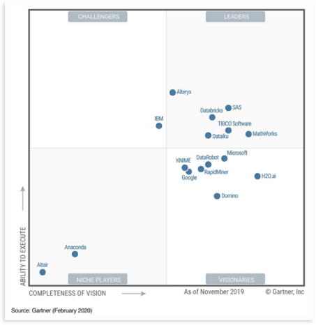
Then the silence for about a century, up to Markov, that many will know, if only because seen in the design of telecommunications networks and much more, including the analysis of texts and natural language.

Then for another half century another silence; meanwhile the greatest scientist of the era, Alan Turing, was working on the “war”. But at the end of this dark period, he gave life to what will be the foundation of the analysis of the data in modern key: neural networks. In those years, the production of transistors on an industrial scale and the consequent increase in the computational capabilities of computers made it possible to implement most of the algorithms deriving from game theory. It is no coincidence that one of the main pitfalls of computer designers of the last century was to be able to beat the chess world champions. And IBM did it for the first time in 1996.

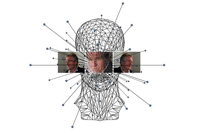
But let’s get back to us, precisely in the 70s, when the foundations were laid for the backpropagation algorithms that have evolved up to the present day in the Generative Adversarial Networks (GANs). By the way, I strongly advise you to read the contents of the MIT website which explains the basics of what is most advanced today in the field of research: http://introtodeeplearning.com/, especially as regards the generation of the so-called “Deep Fake” . If you want to know, for example, which of these faces is real and which is artificially generated, go to the indicated link and find out.
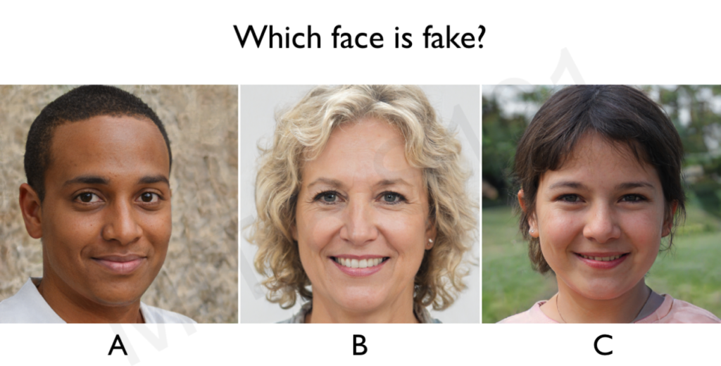
6S191_MIT_DeepLearning_L4

Finally, the news of the experimentation in the context of the Sync project, which has created the prototype of an elementary hybrid network of three neurons, one biological and two artificial, in the field of Bio Medicine, is just these days.

If you have already done so and you are updated and aware, you will have wondered what the ethical limit is for all these applications. Right now I don’t have an answer, but a suggestion: there is a way to deceive the calculators and it is contained in the link above.

Let’s go back to our goal: is it really useful to apply stacking and voting to our learning algorithm? Before expressing an evaluation and some experimental results, let’s remember the definitions. Stacking is the combination of several models in succession to improve the results of machine learning, while voting and averaging are two ensemble methods: voting is used for classification and the average is used for regression and in practice they select the value. of the target variable (both for classification and for prediction) based on the greater number of votes expressed by the algorithms used.
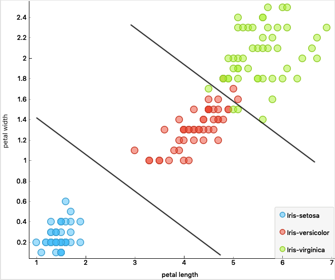
Iris Dataset

Attributes: width and length petal and sepal ; 150 instances

A good mathematician would answer this question: “it depends on the input data”, and therefore we follow the same procedure. Before starting, however, let’s summarize what is the problem of classification and, therefore, of prediction. And let’s start from the first and most famous public domain dataset: Iris, dated 1936, which describes a set of Iris flowers of three different species, which therefore have individually different characteristics according to four parameters.

The classification can take place, for example, by defining a “boundary” that can separate the blue samples (the choice of the noun is not accidental), that is iris-silky from iris-versicolor and iris-virginica. In this case a linear border manages to separate the samples quite well and there are only a few “exceptions” or outliers. However, we will always ask ourselves later: is it better to increase the complexity of the model to identify and correct classification errors or do those samples represent exceptions and is it better to focus on why such exceptions occur? If we call these exceptions, or anomalies, for example, with the name “Spam” or “Cyber ​​Attack” we will understand why this is one of the main problems of IT at the moment. If we are good at classifying instances (events), we are also good at predicting the future, or simply at understanding the event better. In the example we have seen, the Adaboost and Random Forest algorithms lead to an accuracy of 97.9%, which means that given an Iris represented only by the four attributes, petal width, petal length, sepal width, sepal length , we can predict with what 97.9% accuracy what type of Iris it is, without seeing it. But without forgetting that that will be a new sample for my dataset (Knowledge Base). Of course we could do the same thing in many different areas, for example trying to predict the quality of a wine based on some attributes such as PH, residual sugar, citric acid, sulphates, etc., without tasting it.

Let’s go back to our models and represent from the side just an example of a stacking model for the evaluation of the classification accuracy starting from data of different nature, both playing with datasets. There are 497 available at this address: https://archive.ics.uci.edu/ml/datasets.php or you can access the European Open Data portal: https://data.europa.eu/euodp/it/ date/
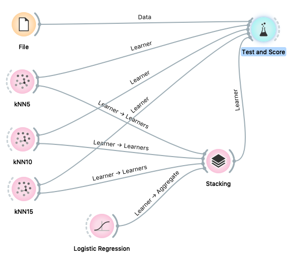
Stacking Model with KNN5, 10 and 15
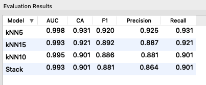
Scores for the Zoo dataset

Zoo animals: dataset size 101 instances, 16 attributes

By injecting different datasets into the model, we find that, in most cases, stacking does not improve the precision of the algorithm used individually, therefore we can say that the goodness of the methodology depends not only on the input data but also on the type of data itself.

With elementary procedure it can be demonstrated, even in the case of voting, that preferring the most accurate model leads to higher accuracy than relying on the results obtained by the majority of the algorithms used, especially for the identification of anomalies.

Another matter, however, the methodologies used in the Convolutional Neural Networks (CNN), for example, for the recognition of images, which break the problem into different sub-problems and cascade different algorithms to these different sub-problems (see 6S191_MIT_DeepLearning_L3) .

I close this article in the hope of not having bored the more experienced, nor of discouraging the new “followers”; however, the areas of expertise embraced are numerous and I am sure that each of you will find a field of application for data analysis. And we will also see some code and algorithms in the next articles.

G. Fruscio

Machine Learning – AutoML vs Hyperparameter Tuning

This entry is part 2 of 5 in the series Machine Learning

Starting back from where we left, majority voting (ranking) or averaging (regression) among the predictions combine the independent predictions into a single prediction. In most cases the combination of the single independent predictions doesn’t lead to a better prediction, unless all classifiers are binary and have equal error probability.

The test procedure of the Majority Voting methodology is aimed at defining a selection algorithm for the following steps:

  • Random sampling of the dataset and use of known algorithms for a first selection of the classifier
  • Validation of the classifier n times, with n = number of cross-validation folds
  • Extraction of the best result
  • Using the n classifiers to evaluate the predictions, apply the selector of the result expressed by the majority of the predictions
  • Comparison of the output with the real classes
  • Comparison of the result with each of the scores of the individual classifiers

Once the test has been carried out on a representative sample of datasets (not by number but by nature), the selection of the algorithm will be implemented and will take place in advance at the time of acquisition of the new dataset to be analysed.

First of all, the selection of the most accurate algorithm, in the event that there is a significant discrepancy on the accuracy found on the basis of the data used, certainly leads to the optimal result compared to the use of a majority voting algorithm which selects the result of the prediction in based on the majority vote (or the average in the case of regression).

If, on the other hand, the accuracy of the algorithms used is comparable or the same algorithm is used in parallel with different data sampling, then one can proceed as previously described and briefly reported below:

  • Random sampling of the dataset and use of known algorithms for a first selection of the classifier
  • Validation of the classifier n times, with n = number of cross-validation folds
  • Extraction of the best result
  • Using the n classifiers to evaluate the predictions, apply the selector of the result expressed by the majority of the predictions
  • Comparison of the output with the real classes
  • Comparison of the result with each of the scores of the individual classifiers

Below is the test log.

Target 5 bins

Accuracy for Random Forest is: 0.9447705370061973
— 29.69015884399414 seconds —
Accuracy for Voting is: 0.9451527478227634
— 46.41354298591614 seconds —

Target 10 bins

Accuracy for Random Forest is: 0.8798219989625706
— 31.42287015914917 seconds —
Accuracy for Voting is: 0.8820879630893554
— 58.07574200630188 seconds —

As can be seen, the improvement obtained compared to the models obtained with pure algorithms is between 0.1% and 0.5%.

Auto-ML vs Hyperparameters Tuning

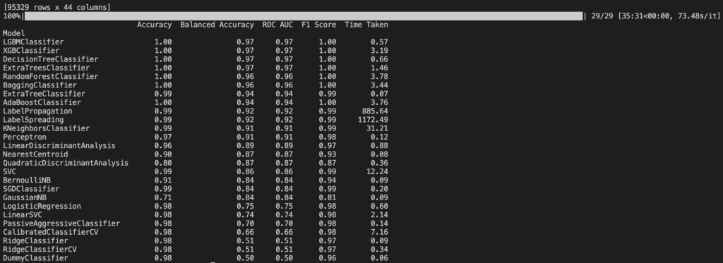
We have used a python library called “Lazy Classifier” which simply takes the dataset and tests it against all the defined algorithms. The result for a 95k rows by 44 columns dataset (normalized log of a backdoor malware vs normal web traffic) is shown in the figure below.

Lazy classifier for Auto-ML algorithm test

It can be noted that picking the best algorithm would result in some cases in an improvement of several percent points (e.g. Logistic Regression vs Random Forest) and, in most cases, in savings in terms of computation time thus consumed energy. For example if we take Random Forest algorithm and we compare the computation with standard parameters and optimization obtained with Grid Search and Random Search, you can notice that the improvement is, again, not worth the effort of repeating the calculation n-times.

**** Random Forest Algorithm standard parameters ****
Accuracy: 0.95
Precision: 1.00
Recall: 0.91
F1 Score: 0.95

**** Grid Search ****
Best parameters: {‘max_depth’: 5, ‘n_estimators’: 100}
Best score: 0.93
**** Random Search ****
Best parameters: {‘n_estimators’: 90, ‘max_depth’: 5}
Best score: 0.93

Precise information filtering deriving from laws present in nature

This entry is part 3 of 5 in the series Machine Learning

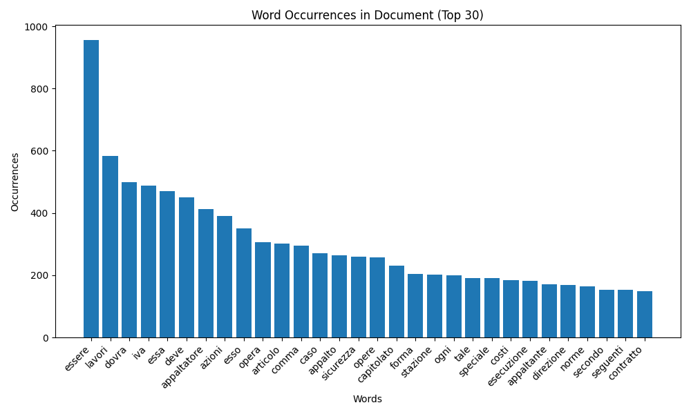
When the probability of measuring a particular value of some quantity varies inversely as a power of that value, the quantity is said to follow a power law, also known variously as Zipf’s law or the Pareto distribution (1). Looking at the figures, it’s really astonishing how most of the information is carried by such a low pecentage of words in a text.

Having in mind other objectives, C. Shannon dedicated most of his life and research to pieces of work that became fundamental for the Information Theory, and the final results allow to understand what is the acceptable loss of information in order to transfer a sequence of signals in an efficient way.

We have transposed the two approaches in order to perform a deterministic research in text by filtering the total words in a number of texts of the same kind by identifying the keywords of an ontological map built for the purpose.

We allowed the human to perform reinforcement learning on the submitted text and after a very low number of iterations we got incredible results.

In about 88% of cases it was possible to identify exactly the piece of information we were looking for and in all cases we were able to identify the two or three sentences that contained the information, out of documents exceeding the 130 pages in length.

This approach, being a “weak AI” achievement, exploits the following advantages:

  • it uses certain, trackable and validated data sources;
  • it obtains certain results, not probabilistic, not using generative AI;
  • it relies on the ability of the domain expert for reinforcement learning;
  • the knowledge base can be kept in-house and will represent a corporate asset.

(to be continued)

By A. Ballarin, G.Fruscio

The Zipf-Mandelbrot-Pareto law is a combination of the Zipf, Pareto, and Mandelbrot distributions. It is a power-law distribution on ranked data that is used to model phenomena where a few events or entities are much more common than others. The probability mass function of the Zipf-Mandelbrot-Pareto law is given by a power-law distribution on ranked data, similar to Zipf’s law. The Zipf-Mandelbrot-Pareto model is often used to model co-authorship popularity, insurance frequency, vocabulary growth, and other phenomena (2,3,4,5)
Applications of the Zipf-Mandelbrot-Pareto law include modeling the frequency of words in a corpus of text data, modeling income or wealth distributions, and modeling insurance frequency. The Zipf-Mandelbrot-Pareto law is also used in the study of vocabulary growth and the relationship between the Heaps and Zipf Laws (2,3,4,5)
Overall, the Zipf-Mandelbrot-Pareto law is a useful tool for modeling phenomena where a few events or entities are much more common than others. It has applications in linguistics, economics, insurance, and other fields (2,3,4,5)

  1. http://www.cs.cornell.edu/courses/cs6241/2019sp/readings/Newman-2005-distributions.pdf
  2. https://eforum.casact.org/article/38501-modeling-insurance-frequency-with-the-zipf-mandelbrot-distribution
  3. https://www.r-bloggers.com/2011/10/the-zipf-and-zipf-mandelbrot-distributions/
  4. https://journalofinequalitiesandapplications.springeropen.com/articles/10.1186/s13660-018-1625-y
  5. https://www.sciencedirect.com/science/article/pii/S0378437122008172

Timeseries Forecast

This entry is part 4 of 5 in the series Machine Learning

Ancient civilizations, such as the Romans and the Greeks, used various methods for predicting the future. These methods were often based on superstition and religious beliefs. Some of the techniques used by the Romans included divination through chickens, human sacrifice, urine, thunder, eggs, and mirrors. The Ancient Greeks also had a variety of methods, such as water divination, smoke interpretation, and the examination of birthmarks and birth membranes. These practices were deeply rooted in their cultural and religious traditions. A scientific approach (one of many possible) involves the use of Machine Learning. In Machine Learning there are a number of benefits of time series prediction: identifying patternsin data, such as seasonal trends, cyclical patterns, and other regularities that may not be apparent from individual data points. Obviously, the main goal is to predict future data points based on historical patterns, allowing businesses to anticipate trends, plan for demand, and make informed decisions. Finally, it helps in better understanding a data set and cleaning the data by filtering out the noise, removing outliers, and gaining an overall perspective of the data. These methods are widely used in various industries, including finance, economics, and business, to make data-driven decisions and predictions. Time-series prediction work was partially founded on the “Laocoonte” project and was based on the fast training of a large number of ML models, tested in parallel and applied each step with the most accurate model. The prediction module was tested in two specific areas, indicated by the availability of real data and future business opportunities, in particular time series prediction (temperature and stock value prediction), tabular data prediction (churn prediction).
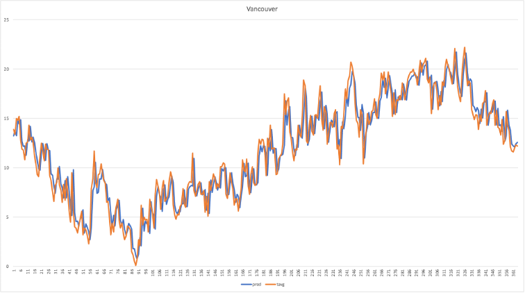
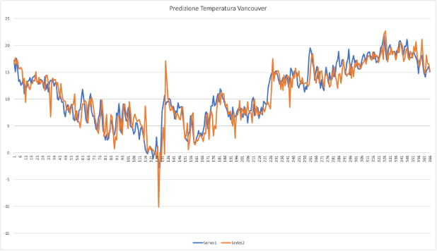
In order to obtain a benchmark against traditional models based on statistical algorithms (ARIMA type), the time series relating to the average daily temperature of Vancouver over the last twenty years was taken as a reference. The sample was subsequently divided in this way:

  • 66% of the samples to train the model;
  • 33% of samples to test the model.
    The result, applied for 365 samples, is shown in the following figure and the measured MAPE (Mean Absolute Percentage Error) is 1.206. The result, applied for 365 samples, is shown in the following figure and the measured MAPE (Mean Absolute Percentage Error) is 1.206.

For the same sample, this time drawn in a different year (September 2004 – September 2005), the result obtained using the Auto-ML predictive model showed a lower performance result, obtaining an MAPE score of 1.647.

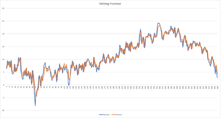
Finally, the SMOreg regression algorithm with 60 lag was applied to the same sample, information on seasonality was introduced and the prediction was carried out using the same train/test ratio. The measured MAPE was 1.2053.

One of the potential applications of the timeseries prediction is forecasting of future values of an underlying, building the model by using historical data. Here below a chart representing a backtest on S&P Future ES-Mini (Equity Line in dollars, maintenance margin 11’200$).