Blog

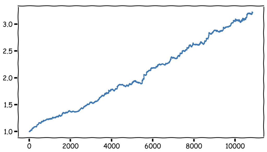
If there is a sport that, in my opinion, can serve well to explain how machine learning works, it’s tennis. Training requires thousands of balls, and it’s estimated that over ten years of practice, more than a million shots are played.

Why, then, do even professional players sometimes miss seemingly easy shots during matches when their error rate in training is often much lower? This is a typical case of overfitting, where the model has been generated from countless balls played, mostly of the same type, hit by the coach or trainer, while during a tournament, players encounter opponents and game situations that are very different—some never seen before.

Styles of play, speed, ball spin, and trajectories can be entirely different from those seen in training. Personally, I think I’ve learned more from matches I lost miserably than from months of training with similar drills. No offense to coaches and trainers—they know it well themselves, having built their experience largely through hundreds of tournaments and diverse opponents.

The similarity with machine learning is quite obvious. Machine learning, like tennis, requires preparation based on experience and the ability to adapt to unforeseen contexts. A model trained on overly homogeneous data may seem very effective during training but fail to recognize new situations—a limitation that only diverse exposure can overcome. Just as a tennis player grows stronger by facing opponents with different styles, a machine learning model improves with data that reflects the variety and complexity of the real world.

In both cases, improvement doesn’t come solely from mechanical repetition but from iterative learning, analyzing errors, and refining strategies. Each mistake, each failure, is a step toward a more resilient and capable system—or player. This is the key to overcoming the limits of overfitting and building skills that go beyond mere memorization, allowing excellence in unexpected conditions.

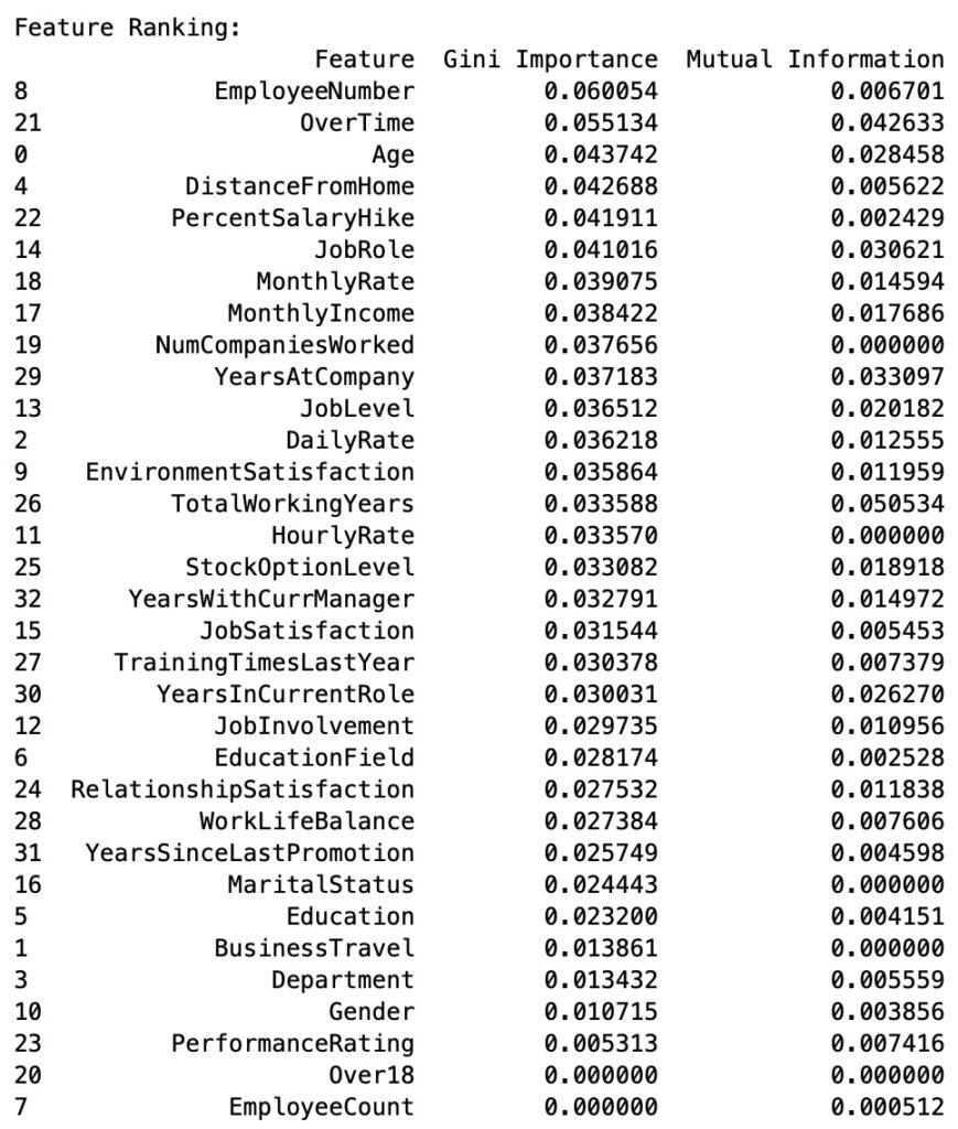
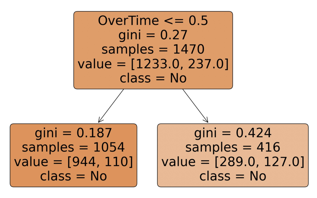
Now let’s move on to the part that interests us the most: biasing. By its nature, an explainable machine learning algorithm (for example, a decision tree) generates models that must “split” on attributes. At some point within the tree (unless the tree’s depth is reduced to avoid this situation), a decision will have to be made based on the value of an attribute, which could lead to discrimination based on gender, age, or other factors.

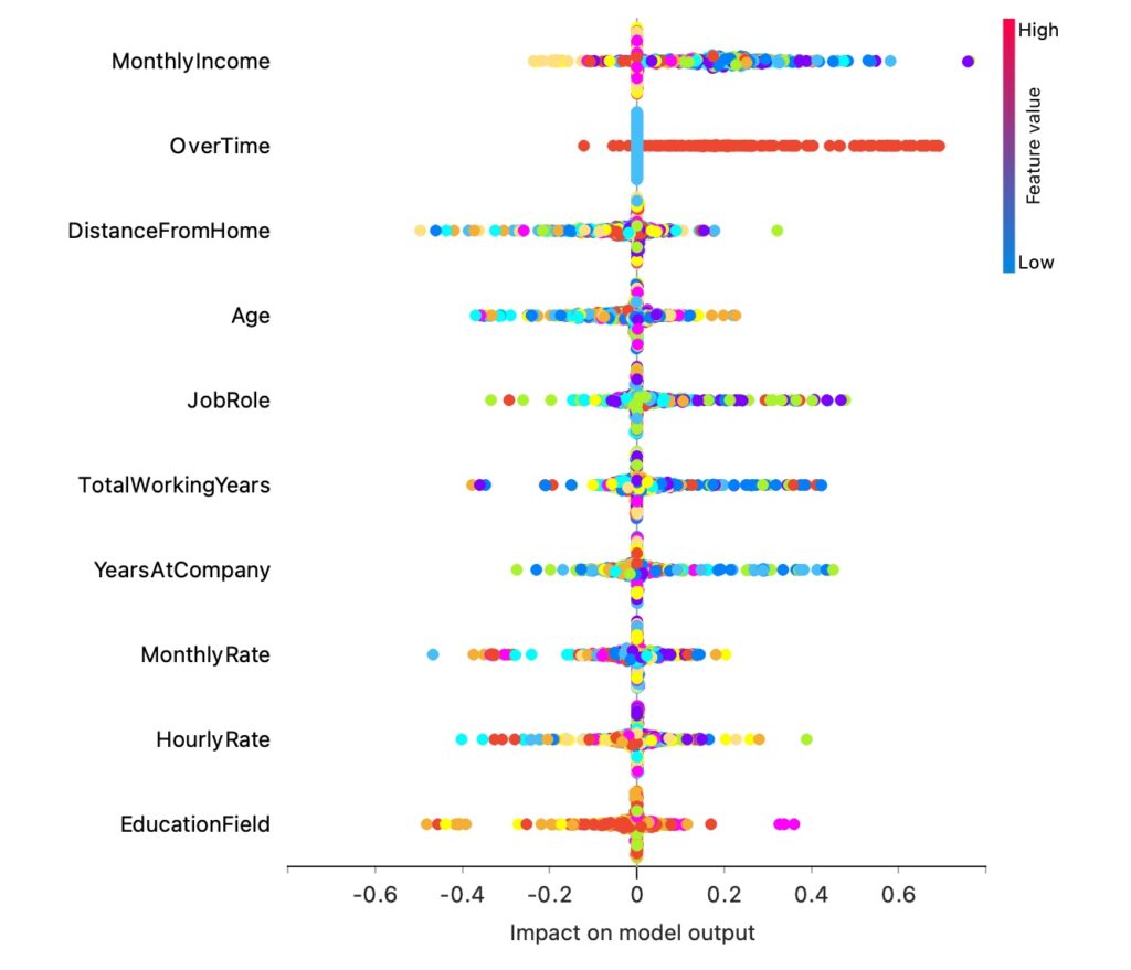
Less explainable algorithms produce results that evaluate all variables simultaneously, thus avoiding decisions based on a single variable. However, there are methodologies (like Shapley values or insights such as those from Antonio Ballarin https://doi.org/10.1063/5.0238654) that allow verification of the impact of a single variable’s variation on a particular target value.

In short, no matter how balanced the dataset is and how low the impact of the observed variable on the target is, there will always be slight biasing in the generated model. A temporary solution, considering the tennis example, is to eliminate the variable that could cause the model to behave in ways deemed unethical (e.g., age, gender, nationality) and construct an initial model that is certainly less accurate than one using all variables but usable from day one.

As the model learns, increasingly de-biased data will be provided (data must be filtered at the source, balancing the number of cases, for instance, between genders). Meanwhile, the algorithm (which at this point won’t know the value of the excluded attribute because it doesn’t exist) will update the model, enabling it to generalize more and more—like an athlete participating in a large number of tournaments.

By now, we are all aware of the potential of AI and, to some extent, the risks associated with its unethical use.

However, I would like to bring attention to a use case that might change the perception of what is ethical and what the definition of ethics entails.

A well-known open dataset from UCI includes the characteristics of employees in a company, and among the attributes, there is a variable that can be used as a target, representing the status of the employee (attrition: yes or no).

The objective could be to pay more attention to employees who, according to the model, appear to be at higher risk of attrition, and this goal might alter the concept of ethics (which, by the way, is not uniform across communities, cultures, or contexts). For example, dataset bias related to attributes like gender or age in this case could help focus more on the disadvantaged groups (here meant as attributes). This is just a different point of view and it doesn’t necessarily mean it’s an ethical approach (e.g. somebody may object that a model built on this data would allow for retaining just resources with high scores in performance reviews).

Below is an analysis of the dataset that highlights some interesting aspects, such as the importance of certain attributes that may not be intuitively significant, or vice versa. For instance, after removing the employee number, which represents an identity, monthly salary ranks only fifth in importance, while gender is among the least important, thus having minimal influence on the target variable.

By breaking down according to the maximum value of Gini impurity 2p*(1-p), a binary tree is constructed in this way and shown in figure.

The second variable to observe is precisely OverTime, which also represents the dependency of attrition on the overtime value recorded for the employee. In this case we use a CNN and shapley values to determine dependence of the target from independent variables.

Finally, we must note that age has strong impact on the decision, but it is quite fragmented and it is selected to separate very well the classes close to the leaves. Here below two examples of clear separation between the two classes.

Edited by G.Fruscio