Autore: Giovanni

Starting back from where we left, majority voting (ranking) or averaging (regression) among the predictions combine the independent predictions into a single prediction. In most cases the combination of the single independent predictions doesn’t lead to a better prediction, unless all classifiers are binary and have equal error probability.

The test procedure of the Majority Voting methodology is aimed at defining a selection algorithm for the following steps:

• Random sampling of the dataset and use of known algorithms for a first selection of the classifier
• Validation of the classifier n times, with n = number of cross-validation folds
• Extraction of the best result
• Using the n classifiers to evaluate the predictions, apply the selector of the result expressed by the majority of the predictions
• Comparison of the output with the real classes
• Comparison of the result with each of the scores of the individual classifiers

Once the test has been carried out on a representative sample of datasets (not by number but by nature), the selection of the algorithm will be implemented and will take place in advance at the time of acquisition of the new dataset to be analysed.

First of all, the selection of the most accurate algorithm, in the event that there is a significant discrepancy on the accuracy found on the basis of the data used, certainly leads to the optimal result compared to the use of a majority voting algorithm which selects the result of the prediction in based on the majority vote (or the average in the case of regression).

If, on the other hand, the accuracy of the algorithms used is comparable or the same algorithm is used in parallel with different data sampling, then one can proceed as previously described and briefly reported below:

• Random sampling of the dataset and use of known algorithms for a first selection of the classifier
• Validation of the classifier n times, with n = number of cross-validation folds
• Extraction of the best result
• Using the n classifiers to evaluate the predictions, apply the selector of the result expressed by the majority of the predictions
• Comparison of the output with the real classes
• Comparison of the result with each of the scores of the individual classifiers

Below is the test log.

Target 5 bins

Accuracy for Random Forest is: 0.9447705370061973
— 29.69015884399414 seconds —
Accuracy for Voting is: 0.9451527478227634
— 46.41354298591614 seconds —

Target 10 bins

Accuracy for Random Forest is: 0.8798219989625706
— 31.42287015914917 seconds —
Accuracy for Voting is: 0.8820879630893554
— 58.07574200630188 seconds —

As can be seen, the improvement obtained compared to the models obtained with pure algorithms is between 0.1% and 0.5%.

Auto-ML vs Hyperparameters Tuning

We have used a python library called “Lazy Classifier” which simply takes the dataset and tests it against all the defined algorithms. The result for a 95k rows by 44 columns dataset (normalized log of a backdoor malware vs normal web traffic) is shown in the figure below.

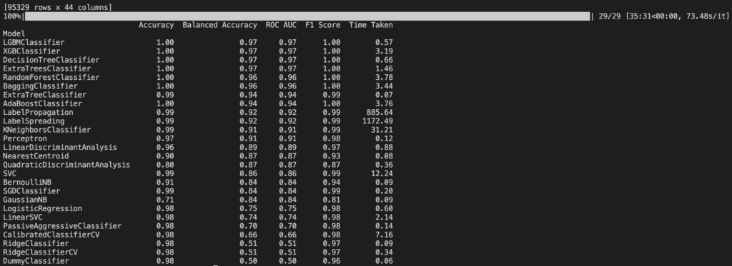
It can be noted that picking the best algorithm would result in some cases in an improvement of several percent points (e.g. Logistic Regression vs Random Forest) and, in most cases, in savings in terms of computation time thus consumed energy. For example if we take Random Forest algorithm and we compare the computation with standard parameters and optimization obtained with Grid Search and Random Search, you can notice that the improvement is, again, not worth the effort of repeating the calculation n-times.

**** Random Forest Algorithm standard parameters ****
Accuracy: 0.95
Precision: 1.00
Recall: 0.91
F1 Score: 0.95

**** Grid Search ****
Best parameters: {‘max_depth’: 5, ‘n_estimators’: 100}
Best score: 0.93
**** Random Search ****
Best parameters: {‘n_estimators’: 90, ‘max_depth’: 5}
Best score: 0.93