Ancient civilizations, such as the Romans and the Greeks, used various methods for predicting the future. These methods were often based on superstition and religious beliefs. Some of the techniques used by the Romans included divination through chickens, human sacrifice, urine, thunder, eggs, and mirrors. The Ancient Greeks also had a variety of methods, such as water divination, smoke interpretation, and the examination of birthmarks and birth membranes. These practices were deeply rooted in their cultural and religious traditions. A scientific approach (one of many possible) involves the use of Machine Learning. In Machine Learning there are a number of benefits of time series prediction: identifying patternsin data, such as seasonal trends, cyclical patterns, and other regularities that may not be apparent from individual data points. Obviously, the main goal is to predict future data points based on historical patterns, allowing businesses to anticipate trends, plan for demand, and make informed decisions. Finally, it helps in better understanding a data set and cleaning the data by filtering out the noise, removing outliers, and gaining an overall perspective of the data. These methods are widely used in various industries, including finance, economics, and business, to make data-driven decisions and predictions. Time-series prediction work was partially founded on the “Laocoonte” project and was based on the fast training of a large number of ML models, tested in parallel and applied each step with the most accurate model. The prediction module was tested in two specific areas, indicated by the availability of real data and future business opportunities, in particular time series prediction (temperature and stock value prediction), tabular data prediction (churn prediction).
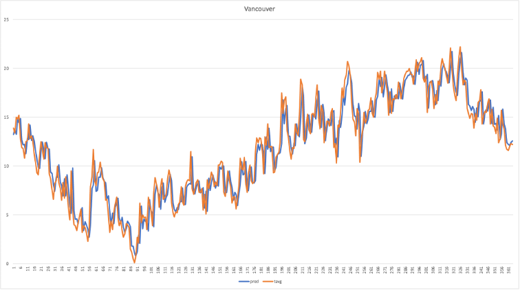
In order to obtain a benchmark against traditional models based on statistical algorithms (ARIMA type), the time series relating to the average daily temperature of Vancouver over the last twenty years was taken as a reference. The sample was subsequently divided in this way:
- 66% of the samples to train the model;
- 33% of samples to test the model.
The result, applied for 365 samples, is shown in the following figure and the measured MAPE (Mean Absolute Percentage Error) is 1.206. The result, applied for 365 samples, is shown in the following figure and the measured MAPE (Mean Absolute Percentage Error) is 1.206.
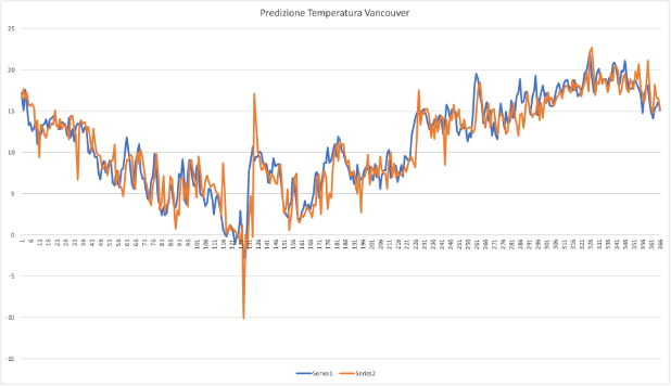
For the same sample, this time drawn in a different year (September 2004 – September 2005), the result obtained using the Auto-ML predictive model showed a lower performance result, obtaining an MAPE score of 1.647.
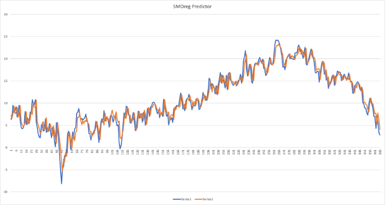
Finally, the SMOreg regression algorithm with 60 lag was applied to the same sample, information on seasonality was introduced and the prediction was carried out using the same train/test ratio. The measured MAPE was 1.2053.
One of the potential applications of the timeseries prediction is forecasting of future values of an underlying, building the model by using historical data. Here below a chart representing a backtest on S&P Future ES-Mini (Equity Line in dollars, maintenance margin 11’200$).